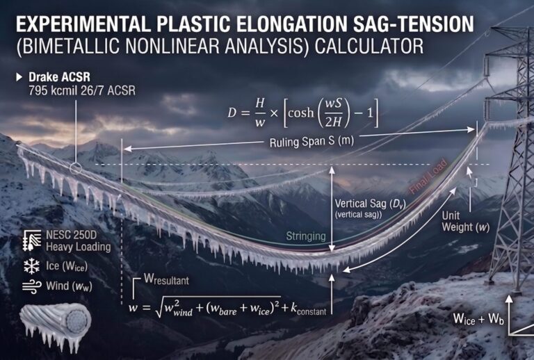
Sag and Tension Calculator with Ice and Wind Loading
Sag and Tension Calculator with Ice and Wind Loading
Pick a conductor, enter your span and stringing tension, and get the final horizontal tension, initial and final sag, and blowout angle under temperature, ice and wind. Every result comes with a step-by-step solution you can check by hand.
Sag and Tension Calculator
Choose a conductor from the list to fill in its properties, or type your own values. Set the initial (stringing) condition, then the final loading condition you want to check, and press Calculate.
What to Enter and What You Get Back
The calculator compares two states of the same span: the day the conductor was strung, and the loading case you are checking.
Which conductors are in the list?
Six ACSR sizes (Sparrow, Quail, Penguin, Linnet, Dove, Condor) and one all-aluminum conductor (Arbutus, 795 kcmil). Selecting one fills in its coefficient of thermal expansion, final modulus of elasticity, area and diameter. The conductor weight and rated strength are taken from the same record. You can overwrite any of the four property fields if your supplier’s data sheet gives different values.
What goes into the initial and final conditions?
- Span (m) — the level span between supports.
- Initial tension (N) — the horizontal tension you string to, usually taken from your stringing chart at the erection temperature.
- Initial temperature (°C) — the conductor temperature at stringing.
- Final temperature (°C) — the case you are checking, such as maximum operating temperature for ground clearance.
- Ice thickness (m) — radial ice on the conductor. Enter it in metres (12.7 mm = 0.0127 m). Set it to 0 for regions with no ice, including the Philippines.
- Wind pressure (N/m²) — pressure on the projected area of the conductor (and ice, if any).
What do the results mean?
- Wice, Wwind, Wresultant — the loads per metre of conductor. The resultant combines the vertical load (conductor plus ice) with the horizontal wind load.
- Blowout angle — how far the conductor swings from vertical under wind. Use it for clearance to structures and between phases.
- A and B — the coefficients of the change-of-state cubic that gives the final tension.
- Final horizontal tension — the tension at the final condition, also shown as a percent of the conductor’s rated strength.
- Initial sag and final sag — catenary sags at the two conditions. Final sag is measured along the plane of the resultant load.
- Final vertical and horizontal sag — the final sag split into its vertical part (for ground clearance) and its sideways part (for swing clearance).
How the Calculator Works
There are three steps: work out the loads, solve the change-of-state equation for the final tension, then compute the sags with the catenary equation.
How are the ice and wind loads calculated?
Variables
w— bare conductor weight, N/m (mass per metre × 9.81)D— conductor diameter, mt— radial ice thickness, mp— wind pressure, N/m²
How is the final tension found?
The calculator uses the parabolic change-of-state equation. The conductor’s length change from temperature and from elastic stretch has to match the change in the geometric length of the curve. Rearranged, that gives a cubic in the final horizontal tension H₂.
Variables
H₁— initial horizontal tension, NS— span, mE,A— final modulus of elasticity (N/m²) and cross-sectional area (m²)α— coefficient of thermal expansion, 1/°Ct₁,t₂— initial and final temperatures, °C
B is always positive, the cubic has exactly one positive root. That root is the final tension, so you never have to choose between solutions.How are the sags calculated?
The initial sag uses the bare weight w and H₁. The final sag uses the resultant load W and H₂. For why the catenary form is used here instead of wS²/8H, see the role of catenary equations in sag and tension.
Worked Example: Dove ACSR on a 300 m Span
These are the same numbers the calculator returns. Enter them yourself to compare.
| Conductor | Dove, 556.5 kcmil 26/7 ACSR |
| w | 1.14238 kg/m × 9.81 = 11.2068 N/m |
| EA | 75.5 × 10⁹ N/m² × 0.0003279 m² = 24,756,450 N |
| α | 1.92 × 10⁻⁵ /°C |
| Span | 300 m |
| Initial | H₁ = 10,000 N at 25 °C |
How much does the sag grow at a higher conductor temperature?
Take a final temperature of 40 °C with no ice and no wind, so W = w.
What happens under a strong wind?
Keep the temperature at 25 °C and apply a wind pressure of 700 N/m². This is an illustration value, not a code requirement. Use the design wind pressure from your governing code.
| Result | Value |
|---|---|
| Wwind | 16.4813 N/m |
| Wresultant | 19.9305 N/m |
| Blowout angle | 55.79° |
| Final horizontal tension | 17,255.50 N (17.3% of rated strength) |
| Final sag (along the resultant) | 13.027 m |
| Vertical sag | 7.325 m |
| Horizontal sag (swing) | 10.772 m |
Limitations and When to Use EPE or SPE
This is a quick check, not a full stringing analysis.
What does this calculator leave out?
- Plastic elongation and creep — ignored. Real conductors stretch permanently over time, which increases final sag.
- Modulus — one final modulus of elasticity is used for the whole conductor. For ACSR, the aluminum and steel layers actually share load differently at high temperature.
- Span geometry — level span only, with supports at the same height.
- Change of state — solved with the parabolic approximation, while the sags use the full catenary. For normal sag-to-span ratios, the difference is small.
Summary of Equations
For the full set of sag-tension formulas, including inclined spans and ruling span, see the sag and tension formulas cheat sheet.