The Role of Catenary Equations in Sag and Tension Calculations
The catenary equation is the backbone of transmission line design — it's the actual shape a conductor takes under its own weight and tension, and it drives every clearance check, sag template, and tower spotting decision that follows. Every shortcut used later, from the parabola to the ruling span, is a simplification of this curve — and knowing where it comes from is what tells you when those shortcuts are safe to use. This post derives it fully, from force balance to final formula.
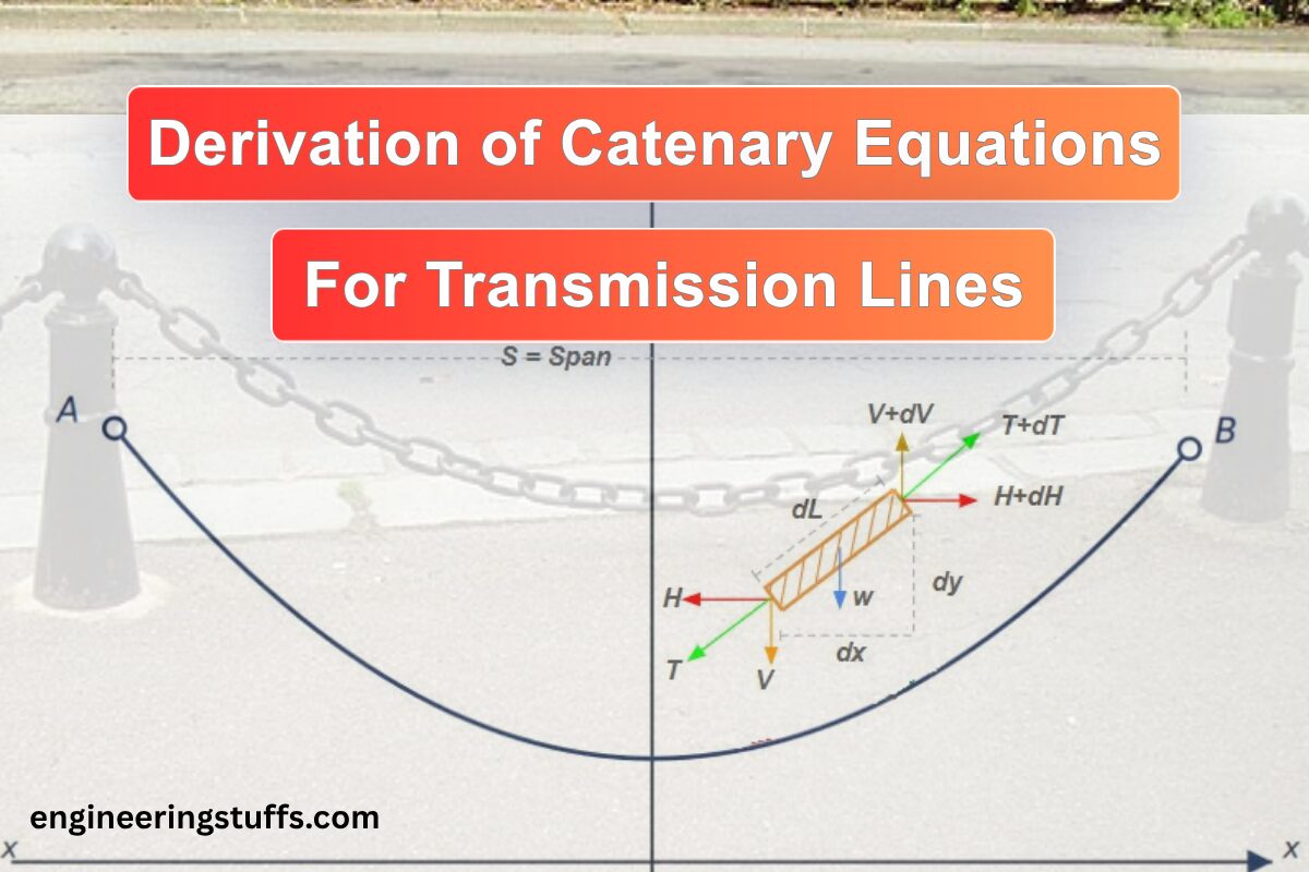
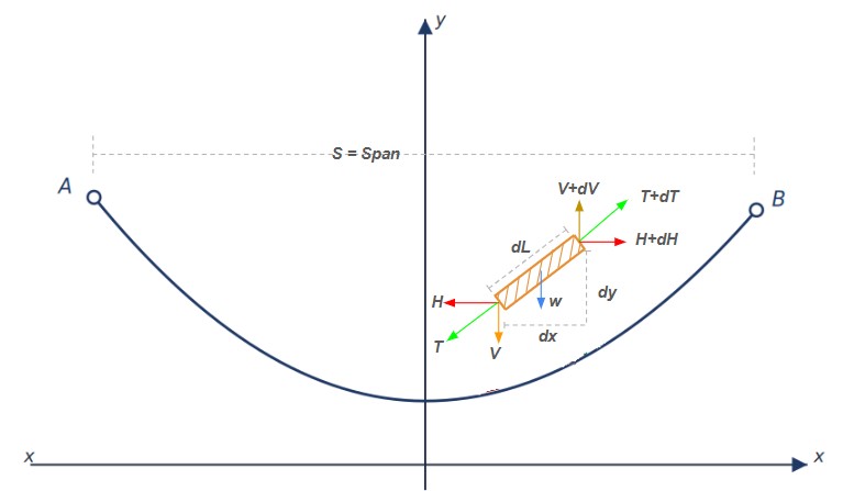
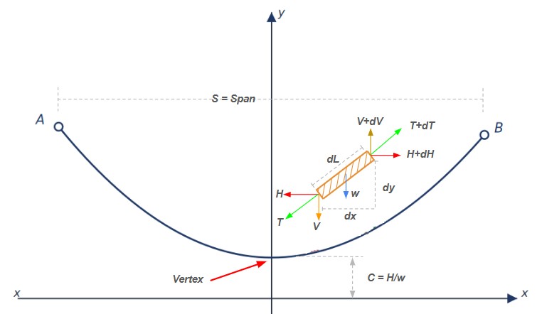
S = span, D = sag, L = conductor length, w = weight per unit length, H = horizontal tension.
The catenary equation appears throughout this site's sag-tension calculators and worked examplesThis post derives it directly, starting from a force balance on an infinitesimal element of conductor and working through every intermediate step, then continues to the sag, maximum sag, and conductor length formulas that follow from it.
| Symbol | Meaning |
|---|---|
H | Horizontal component of conductor tension (constant along the span) |
V | Vertical component of conductor tension (varies along the span) |
w | Conductor weight per unit length |
x, y | Horizontal and vertical coordinates |
dL | Infinitesimal length of conductor |
S | Span length (horizontal distance between supports) |
D | Sag (vertical drop below the line joining the two supports) |
L | Total conductor length between supports |
x₀, y₀ | Constants of integration (coordinates of the origin, fixed in Part 3) |
Let's isolate an infinitesimal segment of conductor, length dL, hanging under its own weight. Three forces act on it: weight w·dL acting downward, tension (H, V) at one end, and tension (H+dH, V+dV) at the other end.
Arc length in terms of the coordinates:
Substituting (2) into (1) and dividing by dx:
No horizontal load acts on the element:
Equation (4) integrates to H = const. The horizontal tension is the same at every point along the span.
Tension in a flexible cable is always directed along the tangent to the curve, so the ratio of vertical to horizontal components equals the local slope:
Differentiate (5) with respect to x. Since H is constant, dV/dx = H·d²y/dx². Substitute into (3):
This is the governing differential equation of the sag curve.
Equation (6) is separable, but it takes a specific trick to get there. Start by dividing both sides by √(1+(y')²):
Multiply both sides by y'·dx:
The left side is the derivative of √(1+(y')²), verified directly by the chain rule:
Since y'·dx = dy, equation (6b) is equivalent to:
Both sides are exact differentials. Integrating:
C is undetermined at this stage; no boundary condition has been applied. Write C = -(w/H)y_0, defining a new constant y_0 := -CH/w. This is a valid algebraic substitution since w/H ≠ 0. Equation (6e) becomes:
Equation (7) is separable. Substituting p = (w/H)(y-y_0), dy = (H/w)dp:
Integrating (the left side is the definition of cosh⁻¹), and introducing a second constant x₀:
Solving for y:
Two constants, x₀ and y₀, matching the order of the differential equation. This is the general solution for any coordinate origin.
Let's find the vertex. It's the point of zero slope:
Differentiating (10) gives y' = sinh[(w/H)(x-x₀)], which is zero exactly at x = x₀. The vertex is located at x = x₀. Substituting into (10):
Equation (12) holds for any choice of origin. Setting x₀ = 0 and y₀ = 0 places the origin directly below the vertex. Equation (10) reduces to:
By (12), with y₀ = 0, the vertex sits at height H/w above this origin, not at y = 0. The quantity c = H/w is the catenary parameter; the standard form y = c·cosh(x/c) has its vertex at height c, consistent with (12).
Now for the shortcut most engineers actually reach for. For typical span lengths and sags in overhead line design, the slope dy/dx stays small enough that (dy/dx)² ≪ 1. Under this condition, (6) reduces to:
Integrating once, and applying the vertex condition dy/dx = 0 at x = 0:
Integrating again, with the parabola's own vertex placed at y = 0:
Equation (16) is the parabolic approximation to the sag curve, measured as height above the vertex. It was derived independently of the catenary solution. The connection between the two is established by expanding cosh in equation (13) as a Taylor series around x = 0:
The first term, H/w, is the vertex height from (12). Subtracting it — that is, measuring height above the vertex, the same reference used in (16) — leaves:
The leading term of (18) is identical to (16). The parabola is the small-slope limit of the catenary; the terms omitted in (14) are exactly the higher-order terms of this series. Their relative size, and therefore the accuracy of the approximation, depends on wS/H — larger for longer spans or slacker conductors, negligible for typical transmission spans.
Here's a subtlety worth catching early: equation (13) gives height relative to the vertex, not sag. Sag is the vertical drop below the straight line connecting the two support attachment points, A and B.
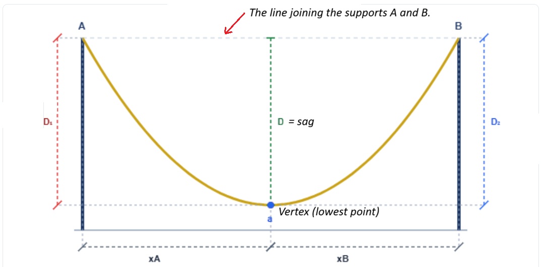
Let support A sit at horizontal position x_A (measured from the vertex), support B at x_B = x_A + S, with height difference h between them. The straight line from A to B has height (h/S)(x-x_A) above A at position x. Sag D is the gap between that line and the curve:
For a level span (h = 0), the vertex sits at midspan, x_A = -S/2. Substituting into (19):
Maximum sag occurs at the vertex (x = 0):
Expanding (21) as a series produces the same structure as (17)–(18): the leading term is wS²/(8H), the parabolic sag formula, with higher-order correction terms from the exact catenary.
One more quantity worth having in closed form: the actual length of conductor between the two supports.
From (7) with the vertex-origin convention, y' = sinh(wx/H), so 1+(y')² = cosh²(wx/H). The square root is exact:
For a level span:
Let's go back to Part 5's vertex position, given only implicitly through equation (16), and solve it in closed form. Using the identity cosh(p) − cosh(q) = 2·sinh((p+q)/2)·sinh((p−q)/2) applied to equation (16):
Equation (25) is exact — not an approximation. Verified numerically against equation (16) across multiple test cases, including negative h (support B lower than A).
x_A < -S/2 or beyond support B). When this happens, the conductor's lowest point on the span is the lower support itself, not a true vertex — the curve is monotonically rising or falling across the whole span. Equation (25) is still mathematically correct in this case; it just describes a point that lies outside the interval actually built.
This is not a corner case worth skipping. It comes up directly in dead-end or angle structures on steep terrain, and in short jumper spans at substations — exactly the spans where a sag template built assuming a mid-span vertex would place the clearance check at the wrong point entirely. Before running a clearance check on a short, steep span, confirm equation (25) actually falls within [-S/2, S/2] first.
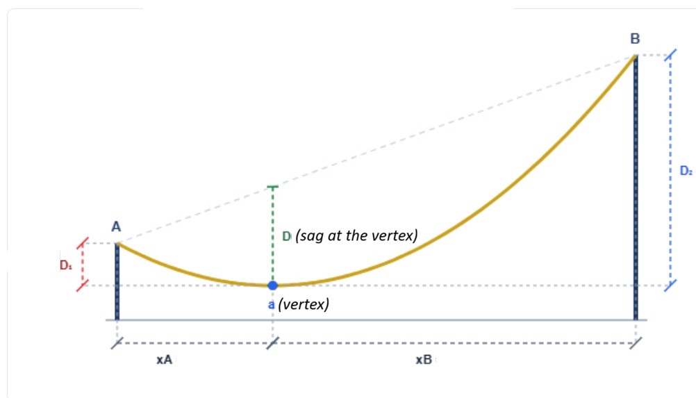
For a level span, maximum sag occurs at the vertex. For an inclined span, it does not — sag is measured relative to the straight line joining the supports, and that line itself is tilted. Differentiating the sag equation (19) with respect to x and setting it to zero:
Solved directly, measuring x from the vertex (not from support A):
Since sinh⁻¹ is an odd, strictly increasing function, x_c has the same sign as h. Maximum sag sits on whichever side of the vertex is closer to the higher support. Verified numerically for positive, negative, and zero h: equation (27) matches the numerically located maximum in every case, to within numerical precision.
sinh⁻¹ in equation (27) — one property of one function, rather than a chain of inequalities.
For hillside spans, this means the governing clearance point is not automatically at midspan or at the vertex — it shifts toward the higher structure. On a sloped profile, checking clearance only at the vertex or only at midspan can miss the actual worst-case point. This is the same effect worked numerically in Problem 4 of the solved-problems post, using the parabolic approximation; equation (27) gives the exact location for the same physical situation.
One last useful quantity: total conductor tension, T = √(H² + V²). Using V = H·sinh(wx/H) from equation (5) and its integrated form:
Comparing to equation (13), H·cosh(wx/H) = w·y, so:
Total tension at any point equals the conductor weight per unit length times the height above the reference line — the same reference line established in Part 3, sitting H/w below the vertex. Verified numerically against the direct calculation of (28) at several positions along the curve.
This gives tension at the support attachment points directly, without separately computing V first — relevant for checking conductor tensile stress against its rated strength at the point where tension is actually highest, which is always at the higher-elevation support, not at the vertex.
T = λgy. Haukaas's UBC lecture notes take yet another route, working with the tangent angle directly instead of dy/dx, and land in the same place.
| Quantity | Formula | Eq. |
|---|---|---|
| Governing differential equation | \( \dfrac{d^2y}{dx^2} = \dfrac{w}{H}\sqrt{1+(dy/dx)^2} \) | (6) |
| General solution (any origin) | \( y = y_0 + \dfrac{H}{w}\cosh\left[\dfrac{w}{H}(x-x_0)\right] \) | (10) |
| Vertex height above the origin | \( y_{\text{vertex}} = y_0 + \dfrac{H}{w} \) | (12) |
| Catenary equation, vertex-origin form | \( y = \dfrac{H}{w}\cosh\left(\dfrac{wx}{H}\right) \) | (13) |
| Parabolic approximation (small slope) | \( y \approx \dfrac{w}{2H}x^2 \) | (16) |
| Sag at any point, unequal-elevation supports | \( D = \dfrac{h}{S}(x-x_A) + \dfrac{H}{w}\left[\cosh\left(\dfrac{wx_A}{H}\right)-\cosh\left(\dfrac{wx}{H}\right)\right] \) | (19) |
| Sag at any point, level span | \( D = \dfrac{H}{w}\left[\cosh\left(\dfrac{wS}{2H}\right)-\cosh\left(\dfrac{wx}{H}\right)\right] \) | (20) |
| Maximum sag, level span | \( D_{max} = \dfrac{H}{w}\left[\cosh\left(\dfrac{wS}{2H}\right)-1\right] \) | (21) |
| Conductor length, general | \( L = \dfrac{H}{w}\left[\sinh\left(\dfrac{wx_B}{H}\right)-\sinh\left(\dfrac{wx_A}{H}\right)\right] \) | (23) |
| Conductor length, level span | \( L = \dfrac{2H}{w}\sinh\left(\dfrac{wS}{2H}\right) \) | (24) |
| Vertex location, inclined span (exact) | \( x_A = \dfrac{H}{w}\sinh^{-1}\left[\dfrac{h}{2\frac{H}{w}\sinh(wS/2H)}\right] - \dfrac{S}{2} \) | (25) |
| Location of maximum sag, from vertex | \( x_c = \dfrac{H}{w}\sinh^{-1}\left(\dfrac{h}{S}\right) \) | (27) |
| Tension at any point | \( T = w\,y \) | (29) |
Equations (1)–(29) derive from one physical fact — constant horizontal tension along the span, equation (4) — combined with calculus. The parabolic approximation in Part 4 is not a separate model; it is the leading term of the exact catenary, verified directly by series expansion in equations (17)–(18). Parts 7 and 8 extend the level-span results to inclined spans and to tension at any point, verified numerically against independent literature. The only place a choice is made rather than derived is the placement of the coordinate origin in Part 3, and that choice is stated explicitly rather than assumed.
References:
Kiessling, F.; Nefzger, P.; Kaintzyk, U.; Nefzger, F.: Overhead Power Lines: Planning, Design, Construction. Berlin, Springer-Verlag, Chapter 14.
Hatibovic, A.: "Derivation of Equations for Conductor and Sag Curves of an Overhead Line Based on a Given Catenary Constant." Periodica Polytechnica Electrical Engineering and Computer Science, 58/1 (2014), 23–27.
Deakin, R.: "Catenary Curve." Dunsborough, WA, Australia, 2019.
Haukaas, T.: "Cables and the Catenary Shape." University of British Columbia lecture notes.