Understanding the EPE Sag-Tension Method (with Interactive Calculator)
Sag-tension calculation is one of those topics that every transmission line engineer encounters but few fully understand at the equation level. Most of us rely on software — and that is entirely appropriate for production design work. But knowing what the software is doing, and why, makes you a better engineer.
In this post I walk through a complete step-by-step calculation for a 300-metre level span using Drake 795 kcmil 26/7 ACSR, following the Experimental Plastic Elongation (EPE) method described in CIGRE Technical Brochure 324 [1] and implemented in PLS-CADD [2]. I then compare the results against PLS-CADD UltraLite v21.04 output to quantify how closely the hand method tracks the software.
Background — The EPE Method in Context
The term EPE stands for Experimental Plastic Elongation (CIGRE TB 324, §6.3 [1]). It refers to the fact that the plastic (permanent) elongation behaviour of the conductor is derived from actual laboratory stress-strain tests, rather than assumed from a composite formula. This matters because aluminum creeps under sustained load, and how much it creeps directly determines the final sags years into service.
To place EPE in context, sag-tension methods can be grouped broadly as follows — following the classification in Alawar et al. [3] and CIGRE TB 324 [1]:
| Method | Catenary | Stress-strain | Notes |
|---|---|---|---|
| NSM (Numerical Sag Method) | Parabolic | Composite E, composite α | Cannot model knee-point [3] |
| HSM / Graphical (SAG10) | Parabolic | Per-component curves | Models knee-point; validated against field data [3] |
| Dong (2015) analytic [4] | Parabolic (approx) | Per-component 4th-order polynomial | Single equation in H; solvable in Excel |
| EPE (this post) | Exact hyperbolic | Per-component 4th-order polynomial | Most accurate; used in PLS-CADD [2] |
The key improvement of EPE over the simpler methods is twofold: it uses the exact hyperbolic catenary (Winkelman [5] noted that parabolic approximations can be “appreciable” in error for long spans or steep inclined spans), and it tracks the per-component thermal and mechanical behaviour of the aluminum outer strands and steel core independently. The NSM, by contrast, uses a single composite thermal coefficient which cannot reproduce the bilinear sag-temperature behaviour observed in ACSR above the knee-point [3].
The Governing Equations
Catenary arc length
A conductor of uniform weight w hanging between two level supports separated by span S forms a catenary. Its arc length is (Winkelman [5], Eq. 2):
The midspan sag is:
Stress-strain polynomial
Each material group (outer aluminium, steel core) has its mechanical stress described by a 4th-order polynomial in mechanical strain ε:
Four curves are used — two for initial loading (O-I) and two for the 10-year creep state (O-C):
| Curve | Material | Condition |
|---|---|---|
AL_I | Outer aluminium | Initial loading |
AL_C | Outer aluminium | After 10 years creep |
ST_I | Steel core | Initial loading |
ST_C | Steel core | After 10 years creep |
How H is determined — the catenary–polynomial intersection
The horizontal tension H is not computed from a formula — it is the solution to three simultaneous conditions. First, the catenary arc length must equal the strained conductor length:
where LREF is the unstressed reference length (derived at installation) and etotal is the total elongation in %. Second, the mechanical strains for each component are found by removing the thermal component, per Dong [4] Eq. (6) and CIGRE TB 324 [1]:
Third, the component stresses must balance the total horizontal tension:
There is no closed-form solution to this system (except under the parabolic approximation as shown by Dong [4]). The exact solution requires an iterative numerical solve — the approach used here and in PLS-CADD [2].
Conductor Data — Drake 795 kcmil 26/7 ACSR
Wire properties are taken from the publicly available Drake ACSR wire file on powline.com, as loaded into PLS-CADD. The polynomial coefficients are sourced from the same file, consistent with Alcoa stress-strain test data [6].
| Property | Symbol | Value | Unit |
|---|---|---|---|
| Cross-section area | A | 468.644224 | mm² |
| Unit weight | w₀ | 15.9657 | N/m |
| Diameter | D | 28.1432 | mm |
| Rated tensile strength | RTS | 140,119 | N |
| Outer modulus (×total A) | EFO | 441.264 | MPa/100 |
| Core modulus (×total A) | EFC | 255.106 | MPa/100 |
| Outer thermal coeff. | αO | 0.002304 | /100°C |
| Core thermal coeff. | αC | 0.001152 | /100°C |
| Reference temperature | TR | 21.1111 | °C (= 70°F) |
Polynomial coefficients (MPa/100)
| Curve | C₀ | C₁ | C₂ | C₃ | C₄ |
|---|---|---|---|---|---|
| AL_I | −8.36333 | 305.493 | −96.5568 | −259.367 | 211.503 |
| AL_C | −3.75626 | 147.732 | −129.912 | 37.8866 | 0 |
| ST_I | −0.477806 | 266.337 | 27.5659 | −315.179 | 192.308 |
| ST_C | 0.324742 | 249.668 | 84.1255 | −499.124 | 319.489 |
Project Setup
| Parameter | Value |
|---|---|
| Span S | 300 m (level) |
| Sagging tension H₀ | 25,000 N at T = 15°C |
| Loading standard | NESC 2017 — Warm Islands |
| Ice density ρice | 8,796.9 N/m³ |
| Wind drag coefficient Cd | 1.0 |
| Creep weather case | 100°C bare wire (212°F) |
Step 1 — Unstressed Reference Length (LREF)
LREF is the conductor length at zero tension and reference temperature TR. It is analogous to the variable eR in Dong [4] (his Eq. 13) and to the “unstressed length” concept in Winkelman [5]. All subsequent weather case calculations refer back to this single value.
1a. Thermal slides at Tsag = 15°C
The thermal slide is the free thermal strain between the stringing temperature and TR. The per-component slides are:
Both are negative because 15°C < TR. Crucially, the outer and core slides differ because αO ≠ αC. This per-component treatment is what allows EPE to track the knee-point — something the NSM composite-α approach cannot do [3].
1b. Solve for total elongation
Find etotal such that both components together carry H₀ = 25,000 N :
Solved numerically (Brent’s method):
1c. Arc length and LREF
Step 2 — Permanent Creep Elongation (PC)
Aluminium creeps under sustained load. We evaluate the conductor at the creep weather case (100°C, bare wire) using the O-C polynomials, then unload elastically to find the zero-stress intercept.
2a. Catenary at 100°C, O-C curves
2b. Elastic unloading — permanent set PC
Step 3 — Permanent Load Elongation (PCP)
Mechanical overload events also produce permanent elongation. The controlling load case is the weather case that produces the largest permanent set (PCP). For this project that is WC3 — NESC 250D Concurrent Ice + Wind at −9°C.
Effective unit weight for WC3
Ice radial thickness t = 2.54 cm, wind pressure P = 196.1 Pa:
Step 4 — Three Conditions per Weather Case
With LREF, PC, and PCP established, every weather case is solved for three conditions using the unloading:
Initial
Solve the O-I catenary at (T, w) with LREF — the same simultaneous system as Step 1.
Final After Creep
Solve the catenary twice: once using the O-I polynomial (giving HOI), and once using a linear elastic law shifted right by PC (giving Hlin). The EPE rule takes the minimum:
This min() rule is directly analogous to the “lower of two curves” approach used in the Hybrid Sag Method [3] and described graphically in PLS-CADD Fig. 9.1-3 [2]. At cold temperatures HOI governs; near 100°C the linear-EF path governs.
Final After Load
PCP (1,433.7 µε) is larger than PC (424.4 µε), so the load-shifted EF line gives lower tension — and correspondingly larger sag — at most weather cases.
Results — Selected Weather Cases
| Weather Case | T (°C) | w (N/m) | Initial | Final / Creep | Final / Load | |||
|---|---|---|---|---|---|---|---|---|
| H (N) | Sag (m) | H (N) | Sag (m) | H (N) | Sag (m) | |||
| Cold bare (−29°C) | −29 | 15.97 | 30,858 | 5.82 | 30,728 | 5.85 | 26,883 | 6.69 |
| Warm bare (16°C) | 16 | 15.97 | 24,942 | 7.21 | 24,852 | 7.23 | 21,825 | 8.24 |
| Hot bare (100°C) | 100 | 15.97 | 18,570 | 9.69 | 18,341 | 9.81 | 17,967 | 10.01 |
| 250D Ice+Wind (−9°C) | −9 | 55.74 | 64,070 | 9.80 | 64,070 | 9.80 | 64,070 | 9.80 |
- Cold bare (−29°C): Initial ≈ Final/Creep because at low temperatures the conductor stress is well above the creep crossover — the O-I curve governs both. Final/Load sag jumps from 5.82 to 6.69 m, reflecting the PCP from WC3.
- Hot (100°C): Creep is visible — H drops by 229 N (−1.2%), adding 0.12 m of sag. The steel core is carrying nearly all the load at this temperature (near or above the knee-point), consistent with the behaviour described by Alawar et al. [3].
- 250D Ice+Wind: All three conditions are identical because WC3 is the controlling load case — the conductor is already at its maximum load elongation at installation.
Comparison with PLS-CADD UltraLite v21.04
To assess the accuracy of this hand method, I ran the same inputs through PLS-CADD UltraLite v21.04 — the industry-standard software for this type of calculation — and compared results across all 22 weather cases and three conditions. The percentage differences between the hand method and PLS-CADD are:
| Condition | RMS Difference | Max Difference |
|---|---|---|
| Initial | 0.095 % | 0.196 % |
| Final / Creep | 0.308 % | 0.463 % |
| Final / Load | 0.130 % | 0.213 % |
| Overall | 0.201 % | — |
The differences are small but not zero. Several factors likely contribute:
- PLS-CADD’s output report rounds horizontal tension to the nearest integer Newton. On a tension of 25,000 N this alone introduces up to ±0.004% per weather case.
- Minor differences in floating-point arithmetic between a Python implementation and a compiled C++ program accumulate through repeated hyperbolic function evaluations, particularly at the longer weather cases with large ΔT.
- The Final/Creep condition shows the largest deviation (0.308% RMS), which is consistent with the creep O-C polynomial being evaluated near the boundary of its valid strain range.
Interactive Calculator
The calculator below implements the EPE method described in this post. It is provided as a learning and reference tool. You can modify the conductor data, span, stringing condition, and weather cases. Results are computed server-side.
Before using the results for any engineering purpose, you must independently verify them. The site is not liable for errors or omissions. By using this calculator you accept these terms.
References
- CIGRE Working Group B2-12, Sag-Tension Calculation Methods for Overhead Lines, Technical Brochure 324, CIGRE, Paris, June 2007.
- Power Line Systems, PLS-CADD Version 21.00 User’s Manual, §9.1 — Sag-Tension Calculations, Power Line Systems Inc., Madison WI, 2025.
- Alawar, A., Bosze, E.J., and Nutt, S.R., “A Hybrid Numerical Method to Calculate the Sag of Composite Conductors,” Electric Power Systems Research, Vol. 76, pp. 389–394, 2006.
- Dong, X., “Analytic Method to Calculate and Characterize the Sag-Tension of Overhead Lines,” IEEE Transactions on Power Delivery, Vol. 31, No. 5, pp. 2064–2071, DOI: 10.1109/TPWRD.2015.2510318, 2016.
- Winkelman, P.F., “Sag-Tension Computations and Field Measurements of Bonneville Power Administration,” AIEE Transactions on Power Apparatus and Systems, Part III, Vol. 78, Issue 4, pp. 1532–1548, February 1960. Paper 59-900.
- Electrical Technical Committee, Stress-Strain-Creep Curves for Aluminum Overhead Electrical Conductors, The Aluminum Association, Washington DC, 1974.
What’s Next
This post covered the single level span case. The next logical step is the ruling span — the equivalent single span that governs a section of unequal suspension spans. The ruling span formula was first derived by Winkelman [5] from the catenary slack equations and is the basis for every stringing chart used in practice. I’ll cover that derivation and its application in the next post.
Questions or corrections? Drop a comment below.