Step by Step SPE Sag and Tension Iteration
In the SPE / Linear Elongation post I said the catenary-modulus system has to be “solved simultaneously” and then just handed you the answer. That’s fine if you trust the calculator, but it’s not much help if you want to build your own spreadsheet — you need to see the actual convergence, not just the final number. That’s what this post is: the same Drake ACSR example, but with every iteration shown.
The method here — bisection — is deliberately the least clever option available. Newton-Raphson converges faster, but it needs a derivative and is easy to get subtly wrong in a spreadsheet. Bisection needs nothing but the residual itself, which is exactly what Excel’s Goal Seek does internally. If you’ve ever used Goal Seek on a sag-tension formula, this is what it was doing behind the scenes.
The Case We’re Solving
Same conductor and span as the SPE post: Drake 795 kcmil 26/7 ACSR, 300 m level span, strung at 48 MPa (22,495 N) at 15°C, SPE model with PC = 600 µε. We’ll converge on the Final/Creep condition at 100°C — the published answer was H = 15,695 N, D = 11.467 m. That’s the number we’re about to derive from scratch, iteration by iteration.
| Quantity | Value |
|---|---|
| Area A | 468.644 mm² |
| Unit weight w₀ | 15.9657 N/m |
| Composite α | 0.001882 %/°C |
| Composite E (true) | 69,637 MPa |
| T_REF | 21.1111 °C |
| LREF (zero-stress, at T_REF) | 300.3945 m |
| LREF, Final/Creep (PC=600µε applied) | 300.5748 m |
| Target temperature T | 100 °C |
The Two Equations That Have to Agree
Sag-tension iteration exists because two independent descriptions of the conductor’s length have to land on the same number, and only one of them is easy to invert.
Equation 1 — the catenary. Given a horizontal tension H, the physical arc length of a hanging conductor is:
Equation 2 — the stress-strain law. Given the same H, the conductor also stretches elastically from its temperature-adjusted unstressed length:
Both equations describe the same physical length, so at the correct H,
Lcat(H) = Ltarget(H). The problem is
that Lcat(H) can’t be algebraically rearranged to isolate H
— it’s transcendental. So instead of solving for H directly, we guess
an H, compute both sides, and adjust the guess based on which side is
bigger.
Setting Up the Bisection
Define the residual as the difference between the two lengths:
We want the H where f(H) = 0. Bisection needs a starting bracket — two values of H where f(H) has opposite signs, guaranteeing a root lies between them (this is just the Intermediate Value Theorem). Any physically reasonable tension range works as a starting bracket; we don’t need to be clever about it, just wide enough to be safe:
Each iteration: evaluate f at the midpoint, then replace whichever bound has the same sign as the midpoint with the midpoint itself. The bracket halves every time — that’s the entire method.
The Actual Convergence, Iteration by Iteration
Here’s every step, computed exactly as you’d lay it out in an Excel
row-by-row bisection table. Ltarget is
recomputed at every Hmid because it depends on H through
the elastic strain term:
| Iter | H_lo (N) | H_hi (N) | H_mid (N) | L_cat(H_mid) | L_target(H_mid) | Residual f(H_mid) |
|---|---|---|---|---|---|---|
| 1 | 5,000.0 | 40,000.0 | 22,500.0 | 300.56677 | 301.22816 | −0.66139 |
| 2 | 5,000.0 | 22,500.0 | 13,750.0 | 301.51908 | 301.14760 | +0.37149 |
| 3 | 13,750.0 | 22,500.0 | 18,125.0 | 300.87368 | 301.18788 | −0.31420 |
| 4 | 13,750.0 | 18,125.0 | 15,937.5 | 301.13026 | 301.16774 | −0.03748 |
| 5 | 13,750.0 | 15,937.5 | 14,843.8 | 301.30319 | 301.15767 | +0.14552 |
| 6 | 14,843.8 | 15,937.5 | 15,390.6 | 301.21211 | 301.16270 | +0.04940 |
| 7 | 15,390.6 | 15,937.5 | 15,664.1 | 301.17011 | 301.16522 | +0.00489 |
| 8 | 15,664.1 | 15,937.5 | 15,800.8 | 301.14993 | 301.16648 | −0.01655 |
| 9 | 15,664.1 | 15,800.8 | 15,732.4 | 301.15995 | 301.16585 | −0.00590 |
| 10 | 15,664.1 | 15,732.4 | 15,698.2 | 301.16502 | 301.16554 | −0.00052 |
| 11 | 15,664.1 | 15,698.2 | 15,681.2 | 301.16756 | 301.16538 | +0.00218 |
| 12 | 15,681.2 | 15,698.2 | 15,689.7 | 301.16629 | 301.16546 | +0.00083 |
| 13 | 15,689.7 | 15,698.2 | 15,694.0 | 301.16565 | 301.16550 | +0.00015 |
| 14 | 15,694.0 | 15,698.2 | 15,696.1 | 301.16533 | 301.16552 | −0.00018 |
| 15 | Converged | 15,695.0 | 301.16549 | 301.16551 | −0.00002 | |
Fifteen iterations to converge to within 0.02 mm of the arc length — from a bracket that started 35,000 N wide. That’s the trade-off with bisection: it’s foolproof, but every iteration only halves the error. Fifteen rows in a spreadsheet is nothing, so for a one-off hand calculation this is genuinely the easiest method to trust.
A Combined Ice + Wind Case, By Hand
Every case so far has been bare wire — no ice, no wind, so the load per unit length is just w₀. Real weather cases aren’t that simple, and the load itself has to be built up from three separate pieces before you can even set up the H-solve. Let’s do that here for NESC 250B — Heavy District Loading: T = −18°C, 1.27 cm radial ice, 191.5 Pa wind pressure, NESC constant k = 4.38 N/m.
Ice load
Ice adds a weight per unit length based on the ice’s own cross-sectional area (an annulus of thickness t around the bare conductor) and its density:
D here is the bare conductor diameter (28.1432 mm), t is radial ice
thickness (12.7 mm). The (D+t) term is the mean diameter
of the ice annulus — this is the standard thin-ring approximation, not
an exact area integral, but it’s what every sag-tension tool including
PLS-CADD uses.
Wind load
Wind pushes on the iced conductor’s projected diameter, so the
ice thickness shows up here too — this time as 2t since
wind sees the full diameter, not the radius:
Resultant load and the NESC k constant
The vertical component is the bare conductor weight plus the ice weight. The wind load acts horizontally. These combine as a vector:
NESC Rule 250B then adds a constant k directly to this resultant — not as a vector, just a flat addition — to build in a safety margin against gust loading that isn’t otherwise captured:
Solving for H under the combined load
Same bisection method as before, just with wtotal in place of w₀ in the catenary equation, and using the Final/Load condition — creep-shifted LREF (PC=600µε applied), evaluated at T=−18°C:
| Iter | H_lo (N) | H_hi (N) | H_mid (N) | Residual |
|---|---|---|---|---|
| 1 | 10,000.0 | 90,000.0 | 50,000.0 | −0.21728 |
| 2 | 10,000.0 | 50,000.0 | 30,000.0 | +1.02699 |
| 3 | 30,000.0 | 50,000.0 | 40,000.0 | +0.20991 |
| 4 | 40,000.0 | 50,000.0 | 45,000.0 | −0.03154 |
| 5 | 40,000.0 | 45,000.0 | 42,500.0 | +0.08056 |
| 6 | 42,500.0 | 45,000.0 | 43,750.0 | +0.02260 |
| 7 | 43,750.0 | 45,000.0 | 44,375.0 | −0.00492 |
| 8 | 43,750.0 | 44,375.0 | 44,062.5 | +0.00872 |
| 9 | 44,062.5 | 44,375.0 | 44,218.8 | +0.00187 |
| 10 | 44,218.8 | 44,375.0 | 44,296.9 | −0.00154 |
| 11 | Converged | 44,257.8 | +0.00017 | |
Slant sag, slant angle, and vertical sag
The catenary equation always gives sag in the plane the conductor actually hangs in — under wind, that plane is tilted away from vertical, so this is a slant sag, not the vertical clearance value you actually need for ground clearance checks:
To get the true vertical sag, you need the angle the conductor has physically swung away from vertical. This angle comes only from the real physical forces — critically, the NESC k constant is excluded here, since k is a fictitious safety-margin load with no physical direction, not an actual force vector:
Replicating This in Excel
You don’t need to hand-build the bisection table above to check your own spreadsheet — that’s what Goal Seek automates. Set it up like this:
- One cell for H (your changing/guess cell).
-
One formula cell computing
L_cat(H) − L_target(H)exactly as defined above, referencing the H cell. - Data → What-If Analysis → Goal Seek: set the residual cell to 0, by changing the H cell.
Excel’s Goal Seek uses essentially the same bracket-and-narrow logic (technically a secant-method variant, which is why it usually converges in far fewer than 15 steps) — but the underlying idea is identical to what’s in the table above. If you want to see it iteration-by-iteration the way this post does, build the bisection table manually with a fixed starting bracket and a formula row you drag down — that reproduces the table exactly.
For repeated calculations (a full weather-case table, multiple spans), a manual Newton-Raphson setup converges in 4–6 iterations instead of 15, using the derivative dLcat/dH. That’s a heavier setup for a one-off spreadsheet check, though — worth it only if you’re running this across many rows and want the calculation to feel snappy.
What’s Next
Back to the SPE / Linear Elongation post for the full model comparison and the interactive calculator, or ahead to the ruling span post — the next post in the series — for how this single-span math extends to a full line section.
Questions or corrections? Drop a comment below.
References
- CIGRE Working Group B2-12, Sag-Tension Calculation Methods for Overhead Lines, Technical Brochure 324, CIGRE, Paris, June 2007.
- Power Line Systems, PLS-CADD Version 21.00 User’s Manual, §9.1, Power Line Systems Inc., Madison WI, 2025.